Simulation of the Grid
In this chapter the grid can be simulated using the developed python tool.
See the Code
The whole code is available in the GitHub Repository.
import pandapower as pp
from pandapower import networks as pn
from pandapower import plotting as pt
from pandapower.timeseries.data_sources.frame_data import DFData
import pandapower.control as control
import pandapower.timeseries as timeseries
import pandas as pd
from matplotlib import pyplot as plt
from plotly import graph_objs as go

# custom libraries
from scenario import Scenario
from controllable_battery import ControllableBattery
from battery_controller import BatteryController
import pptools as ppt

# suppress annoying warning
import warnings
warnings.simplefilter(action='ignore', category=FutureWarning)
Necessary Preparations
Creating the network
The first step is to create the network:
# create the kerber network
net = pn.create_kerber_vorstadtnetz_kabel_1()
And take a look at it:
figure = pt.simple_plotly(net);
No or insufficient geodata available --> Creating artificial coordinates. This may take some time...
Setting Parameters
As next step, some parameters determining the simulation have to be set:
the resolution of the simulation (minimum 1 minute)
whether to include some BEVs arriving at the same time
whether to set all charging stations to the same nominal power
whether to change the travelled distances
setting the powerfactor of the SLP
whether to activate controlling
and finally setting the controlling parameters
Set the resolution:
The resolution influences the \(\Delta t\) from Equation (5) and thus the granularity of the whole simulation.
resolution = '15min'
Make BEVs arrive at the same time:
This way it is possible to manipulate the arrival statistic depicted Figure 5, allowing it to simulate extreme scenarios, where all the BEVs arrive at the same time.
same_arrival = False

# arrival_time needs to be set in multiples of quarter hours
arrival_time = 46
Change the nominal power of the charging stations:
This way it is possible to manipulate the distribution of the nominal power of the charging stations in Table 4.
same_power = False

# nominal charging power [kW]
loading_power = 11.1
Change the travelled distance:
This makes it possible to adjust the travelled distance of the BEVs described in Table 3, thus determining the state of charge according to Equation (4) when the charging starts.
same_travelled = False

# travelled distance [km]
distance_travelled = 200
Set the powerfactor of the SLP:
This makes it possible to simulate different powerfactors by adding reactive power to the SLP depicted in Figure 3.
cosphi = 0.9
Activate controlling:
This enables the controller.
controlling = False
Set the controlling parameters:
This way the controlling parameters described in Table 5 can be altered.
if controlling:
    ControllableBattery.set_control_params('Ki', 0.5)
    ControllableBattery.set_control_params('Kd', 0.1)
Creating a Scenario
Tip
It is also possible to create new scenarios using
scenario = Scenario(net, <penetration>)
However, this might change the underlying distributions (as the seed used for generating random choices isn’t fixed).
Next choose one of the proposed scenarios. The scenarios satisfy all of the proposed distributions but might be altered by the settings choosen above.
# 'Szenario0', 'Szenario30', 'Szenario50', 'Szenario80' or 'Szenario100'
scenario = Scenario.load_scenario('Szenario80')
# apply the resolution to the scenario
scenario.set_resolution(resolution)
Visualize the Scenario
Take a look at where the charging stations are placed in the net. Nodes with a charging station attached are marked green:
# figure out which buses have a charger
charger_buses = scenario.scenario_data['according bus nr.'].values
figure.add_trace(go.Scatter(x=net.bus_geodata.loc[charger_buses, 'x'],
                             y=net.bus_geodata.loc[charger_buses, 'y'],
                             mode='markers'))
figure.show();
Running the Simulation
Now the simulation can be run:
if same_arrival:
    scenario.set_constant('time of arrival', arrival_time, inplace=True)

if same_power:
    scenario.set_constant('charging power [kW]', loading_power, inplace=True)

if same_travelled:
    scenario.set_constant('distance travelled [km]', distance_travelled, inplace=True)


data_nuernberg = pd.read_csv('Daten/Lastprofil/Nuernberg_absolut_final.csv')

data_nuernberg = ppt.set_simulation_range(data_nuernberg)

baseload = ppt.prepare_baseload(data_nuernberg, net, resolution)

batteries, datasource_bat = ppt.prepare_batteries(net, scenario, resolution)

loads = DFData(baseload)

# compute factor for share of Q out of P with cosphi
faktor = (1/cosphi**2 -1)**0.5

# data_source for reactive Power Q
loads_q = DFData(baseload * faktor)

# data_source for loading curves of BEVs
loads_bat = DFData(datasource_bat)

# creating controllers
load_controler_q = control.ConstControl(net, element='load', variable='q_mvar',
                                      element_index=net.load.index,
                                      data_source=loads_q,
                                      profile_name=net.load.index)

load_controller_bat = BatteryController(net, element='load', variable='p_mw',
                                        element_index=datasource_bat.columns,#loading_data.columns,
                                        data_source=loads_bat, batteries=batteries,
                                       second_ds=loads)

if controlling:
    load_controller_bat.activate_contolling()


# output writer
writer = timeseries.OutputWriter(net, output_path="./",
                                 output_file_type=".csv")

# which variables to log
writer.log_variable(table='res_bus', variable='vm_pu')
writer.log_variable(table='res_line', variable='loading_percent')
writer.log_variable(table='res_trafo', variable='loading_percent')

# simulate timeseries
timeseries.run_timeseries(net)
No time steps to calculate are specified. I'll check the datasource of the first controller for avaiable time steps
Progress: |██████████████████████████████████████████████████| 100.0% Complete
See the Results
First read in the stored results of the simulation:
results_bus = pd.read_csv('res_bus/vm_pu.csv', sep=';')*400
results_trafo = pd.read_csv('res_trafo/loading_percent.csv', sep=';')
results_line = pd.read_csv('res_line/loading_percent.csv', sep=';')

results_bus.index = pd.date_range(start='2020-12-13', freq=resolution,
                                  periods=len(results_bus))

results_line.index = pd.date_range(start='2020-12-13', freq=resolution,
                                  periods=len(results_bus))

results_trafo.index = pd.date_range(start='2020-12-13', freq=resolution,
                                  periods=len(results_bus))

# figure out critical line and bus
crit_bus = ppt.get_critical_bus(results_bus)
print(f'Maximal belasteter Bus: {crit_bus}')

crit_line = ppt.get_critical_line(results_line)
print(f'Maximal belastete Leitung: {crit_line}')

# configure layout of following plots
if int(resolution.rstrip('min')) >= 15:
    marker = 'x'

else:
    marker=None
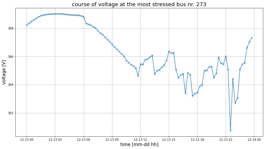
Maximal belasteter Bus: 273
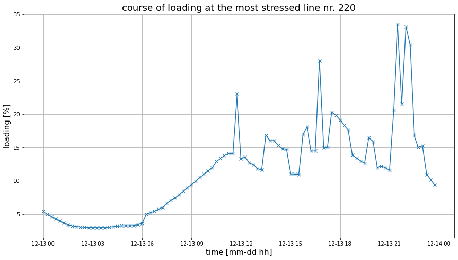
Maximal belastete Leitung: 220
The Bus Voltage
plt.figure(figsize=(15, 8))
plt.plot(results_bus[str(crit_bus)], marker=marker)
plt.title(f'course of voltage at the most stressed bus nr. {crit_bus}', fontsize=18)
plt.ylabel('voltage [V]', fontsize=15)
plt.xlabel('time [mm-dd hh]', fontsize=15)
plt.grid()
The Line loading
plt.figure(figsize=(15, 8))
plt.plot(results_line[str(crit_line)], marker=marker)
plt.title(f'course of loading at the most stressed line nr. {crit_line}', fontsize=18)
plt.ylabel('loading [%]', fontsize=15)
plt.xlabel('time [mm-dd hh]', fontsize=15)
plt.grid()
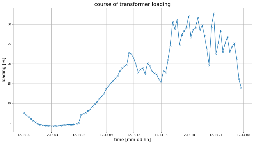
The Transformer Loading
plt.figure(figsize=(15, 8))
plt.plot(results_trafo.iloc[:, 1], marker=marker)
plt.title(f'course of transformer loading', fontsize=18)
plt.ylabel('loading [%]', fontsize=15)
plt.xlabel('time [mm-dd hh]', fontsize=15)
plt.grid()